Learning as a Search
Slope of w Squared at Three
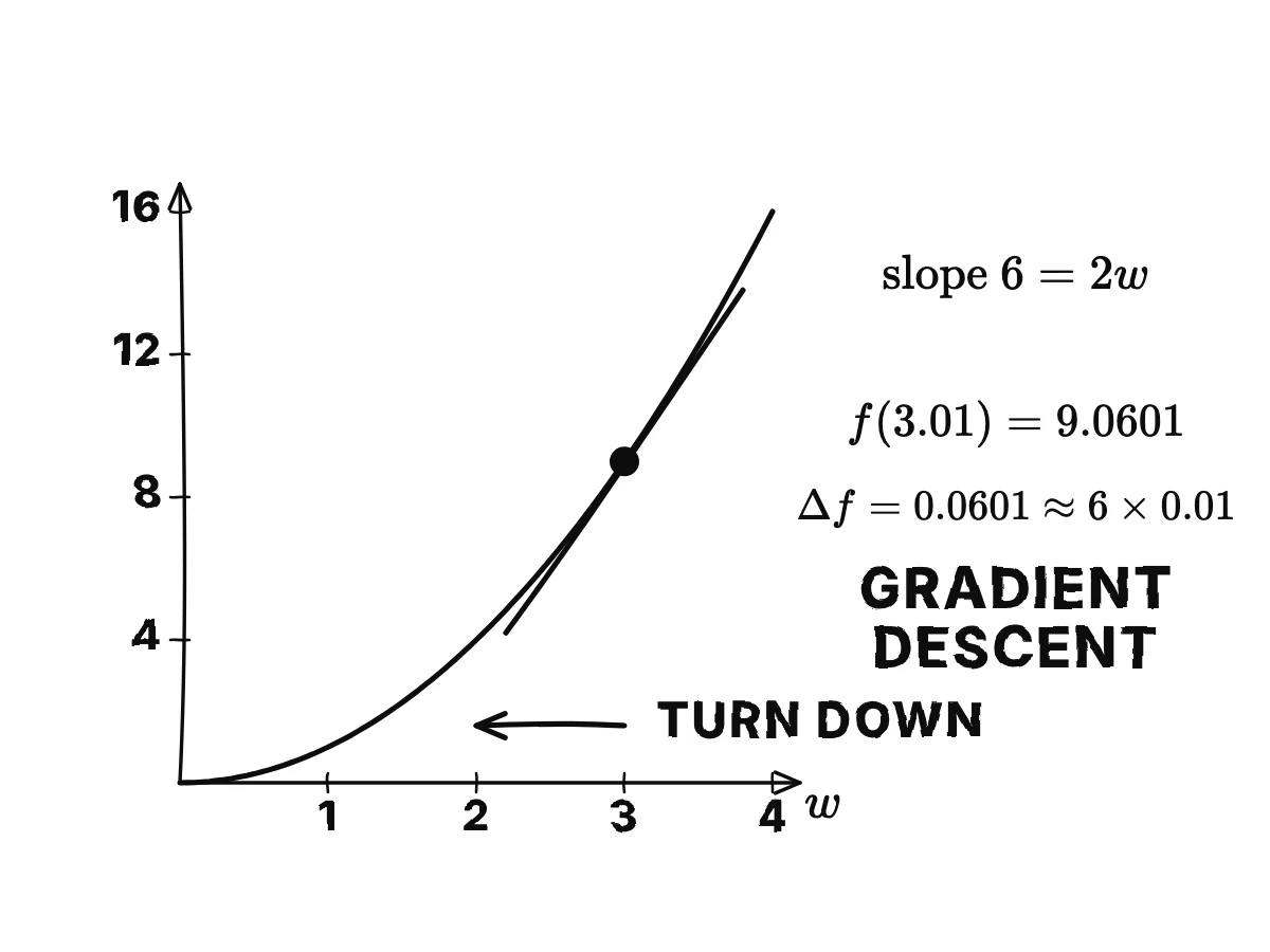
Here is the idea with a single knob and numbers we can check. Suppose the error of a model is f(w) = w², and the knob stands at w = 3, so the error is nine.
Alice's Adventures in a Differentiable Wonderland, Volume I: A Tour of the Land
The same text, told at every level, in every language and look shown here. Pick, then listen or download.
The same player the product gives for your own book: the voice, the drawings as they are drawn, the text.
A modern textbook on how neural networks really work, from tensors and gradients to transformers. The first three chapters lay the ground: what the book is about, the linear algebra and calculus a network runs on, gradient descent, and what a dataset and a loss function are.
This is a sample: 3 of 13 chapters.
Here is the idea with a single knob and numbers we can check. Suppose the error of a model is f(w) = w², and the knob stands at w = 3, so the error is nine.
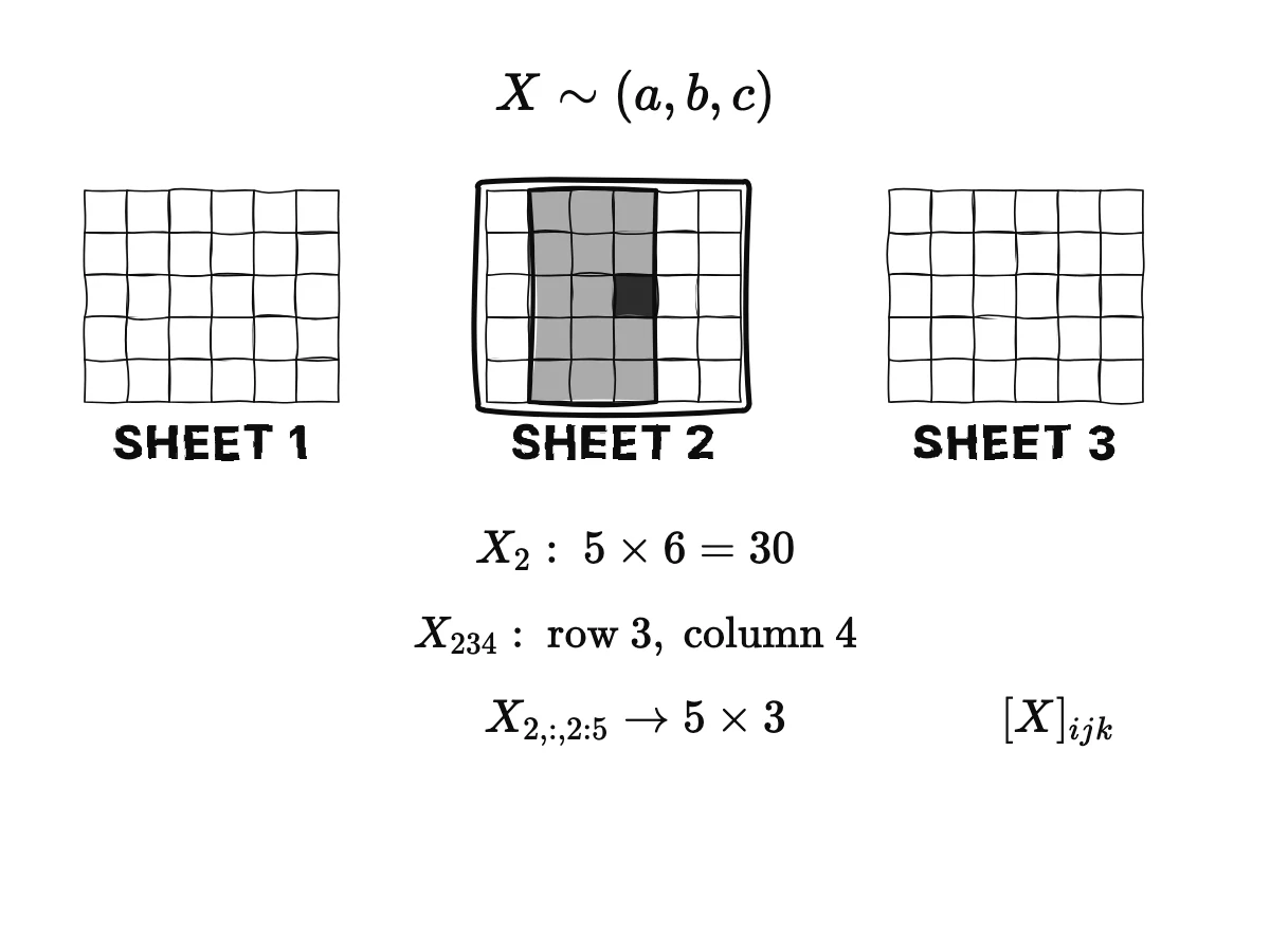
Take a three-dimensional tensor X ∼ (a, b, c). Then Xᵢ is one slice of shape (b, c): in our photo batch, X₂ is the whole second photo, a 5 by 6 grid of 30 numbers. And Xᵢⱼₖ is a single scalar: X₂₃₄ is the brightness of the pixel in row 3, column 4 of the second photo, one crumb of the loaf.
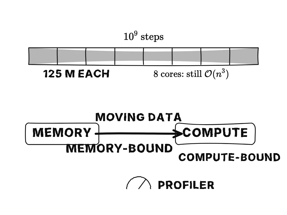
Two more limits of asymptotic thinking. First, having k processors does not change the big-O at all: at best it divides the time by k, a constant factor; eight cores turn a billion steps into 125 million each, still cubic in n.
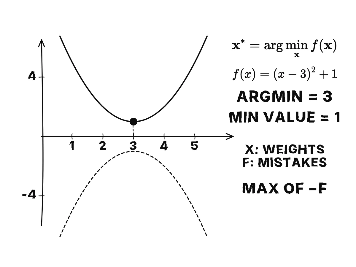
Now the reason gradients are worth all this: section 2.3, gradient descent. The task is to minimize a function f(𝐱) with 𝐱 ∼ (d): 𝐱* = argmin f(𝐱). Like argmax, argmin means "the value of x that gives the lowest possible f".
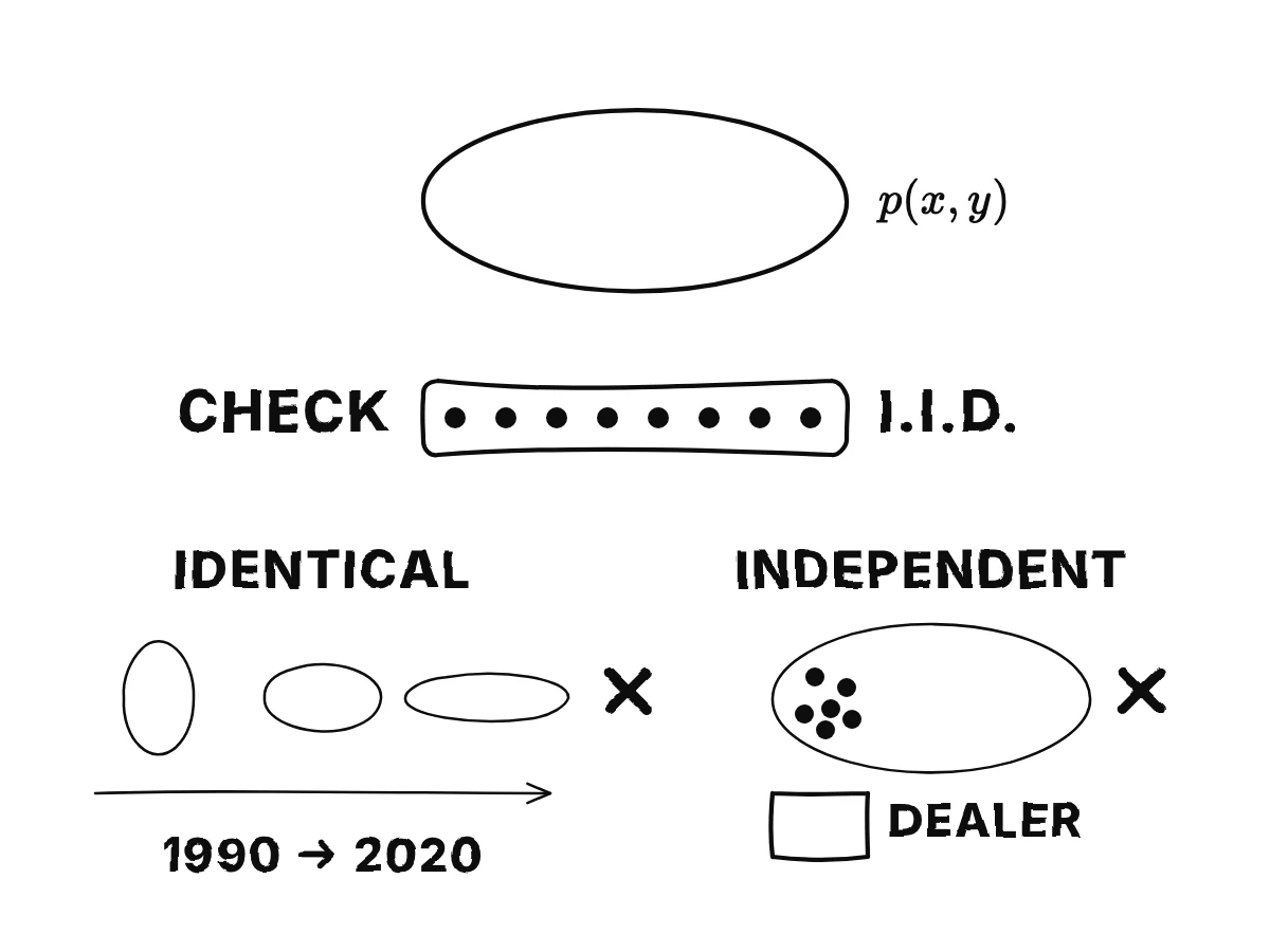
One more assumption is added, and it is crucial: each example is an independent and identically distributed draw, i.i.d., from some unknown, and in fact unknowable, probability distribution p(x, y). It sounds technical, but it is what makes the task meaningful.
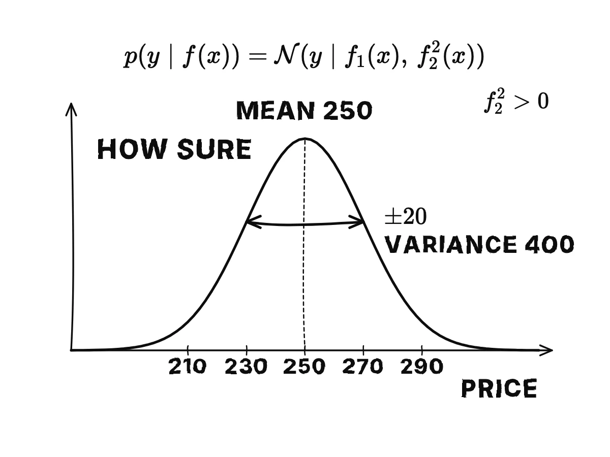
For regression, predicting a real number y ∈ ℝ, the model can output two values, f(x) ∼ (2), the mean and the spread of a Gaussian, a bell curve: p(y ∣ f(x)) = 𝒩(y ∣ f₁(x), f₂²(x)). The second output is squared so that the variance is always positive.
Examples for: a curious adult with school maths who uses AI apps every day; add one modern instance per idea, such as how a chat assistant or a phone's photo app is trained
The lectures retell the English text of arXiv 2404.17625 (version 3, 2025) by Simone Scardapane, published under an open licence that allows retelling and translation. The retelling, the drawings and the voice are made by AI and checked against the book by a second model. How AI is used.
The lectures adapt the original and are released under the same licence, free to share and adapt with credit to the author and a link to this page: CC BY-SA 4.0
Upload a textbook or any difficult book. The first five minutes are free.
Upload a book