Learning as a Search
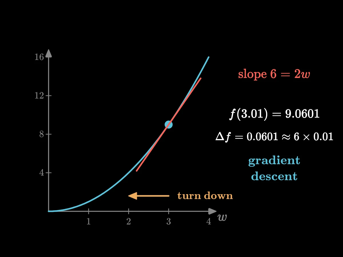
Slope of w Squared at Three
Here is the idea with a single knob and numbers we can check. Suppose the error of a model is f(w) = w², and the knob stands at w = 3, so the error is nine.
Alice's Adventures in a Differentiable Wonderland, Volume I: A Tour of the Land
Один и тот же текст на каждом уровне, на всех языках и во всех оформлениях, что здесь есть. Выберите, потом слушайте или скачивайте.
Тот же плеер, который продукт даёт для вашей книги: голос, рисунки по мере того, как они рисуются, текст.
Современный учебник о том, как на самом деле устроены нейросети: от тензоров и градиентов до трансформеров. Первые три главы закладывают основу: о чём книга, линейная алгебра и анализ, на которых работает сеть, градиентный спуск, что такое набор данных и функция потерь.
Это пробная часть: 3 из 13 (главы).
Here is the idea with a single knob and numbers we can check. Suppose the error of a model is f(w) = w², and the knob stands at w = 3, so the error is nine.
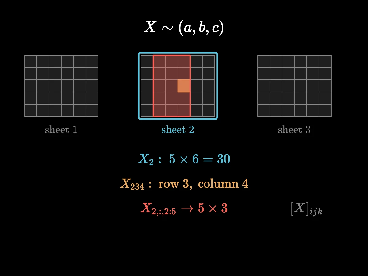
Take a three-dimensional tensor X ∼ (a, b, c). Then Xᵢ is one slice of shape (b, c): in our photo batch, X₂ is the whole second photo, a 5 by 6 grid of 30 numbers. And Xᵢⱼₖ is a single scalar: X₂₃₄ is the brightness of the pixel in row 3, column 4 of the second photo, one crumb of the loaf.
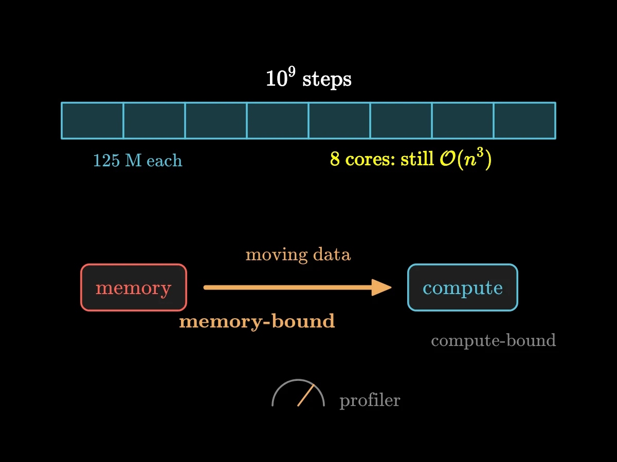
Two more limits of asymptotic thinking. First, having k processors does not change the big-O at all: at best it divides the time by k, a constant factor; eight cores turn a billion steps into 125 million each, still cubic in n.
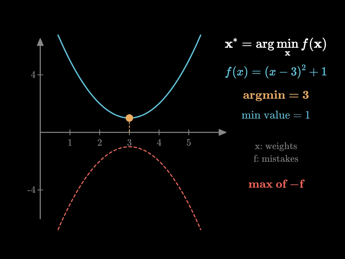
Now the reason gradients are worth all this: section 2.3, gradient descent. The task is to minimize a function f(𝐱) with 𝐱 ∼ (d): 𝐱* = argmin f(𝐱). Like argmax, argmin means "the value of x that gives the lowest possible f".
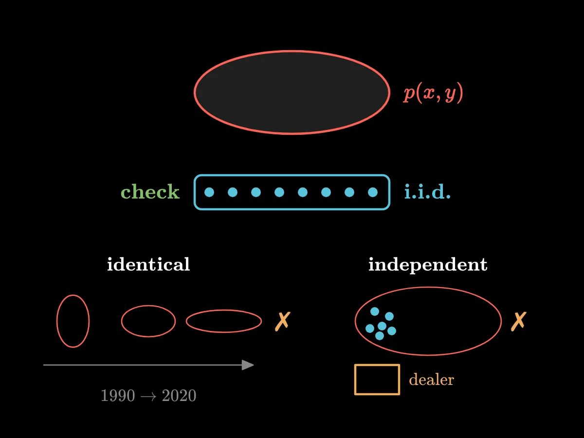
One more assumption is added, and it is crucial: each example is an independent and identically distributed draw, i.i.d., from some unknown, and in fact unknowable, probability distribution p(x, y). It sounds technical, but it is what makes the task meaningful.
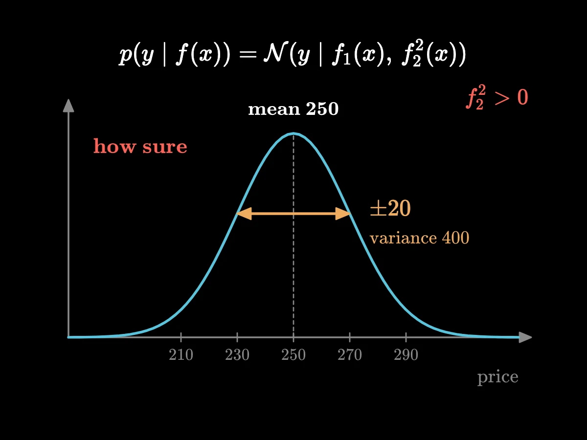
For regression, predicting a real number y ∈ ℝ, the model can output two values, f(x) ∼ (2), the mean and the spread of a Gaussian, a bell curve: p(y ∣ f(x)) = 𝒩(y ∣ f₁(x), f₂²(x)). The second output is squared so that the variance is always positive.
Примеры для: a curious adult with school maths who uses AI apps every day; add one modern instance per idea, such as how a chat assistant or a phone's photo app is trained
Лекции пересказывают с английского оригинала книгу arXiv 2404.17625 (version 3, 2025), автор — Симоне Скардапане; книга вышла под открытой лицензией, которая разрешает пересказ и перевод. Пересказ, рисунки и голос сделаны ИИ и сверены с книгой второй моделью. Как используется ИИ.
Лекции — переработка оригинала и распространяются под той же лицензией: их можно свободно распространять и перерабатывать с указанием автора и ссылкой на эту страницу: CC BY-SA 4.0
Загрузите учебник или любую сложную книгу. Первые пять минут бесплатно.
Загрузить книгу